MImapqtl implements QTL mapping analysis for multiple QTL in
multiple intervals
for a single trait in a single environment. It can begin analysis from an initial model
specifying the positions of QTL, or de novo, that is with no initial model. If given an
initial model, the program will estimate the parameters, refine the estimates of QTL positions within
intervals, test the significance of all parameters, search for more QTL, search for epistatic interactions
and finally calculate the ![]() and breeding values for the model. If analysis is initiated de novo,
then there will be a search for QTL, a search for interactions and calculation of
and breeding values for the model. If analysis is initiated de novo,
then there will be a search for QTL, a search for interactions and calculation of ![]() and breeding values.
MImapqtl can also do a single pass search for a new QTL and create a likelihood ratio profile
for a new putative QTL given any initial model.
and breeding values.
MImapqtl can also do a single pass search for a new QTL and create a likelihood ratio profile
for a new putative QTL given any initial model.
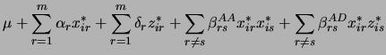
For ![]() putative QTL, the model is
putative QTL, the model is
The likelihood function of the data given the model is a mixture of normal distributions
In (3.7), the ![]() are the probabilities of the multilocus genotypes conditioned on marker data.
The variable
are the probabilities of the multilocus genotypes conditioned on marker data.
The variable ![]() is the number of genotypic classes for the experimental design: For backcrosses and recombinant inbred lines,
is the number of genotypic classes for the experimental design: For backcrosses and recombinant inbred lines,
![]() , while for intercrosses it is
, while for intercrosses it is ![]() . In practice, it is often infeasable to do the
sum over all
. In practice, it is often infeasable to do the
sum over all ![]() multilocus genotypes: We use a subset of the most frequent genotypes. The parameters are in
multilocus genotypes: We use a subset of the most frequent genotypes. The parameters are in
![]() while the coded indicator variables are in
while the coded indicator variables are in ![]() .
.
![]() is the normal density function with mean
is the normal density function with mean
![]() and variance
and variance ![]() . We use an EM (expectation maximization) algorithm to obtain maximum likelihood parameter estimates
[Kao and ZengKao and Zeng1997,Zeng, Kao, and BastenZeng
et al.1999].
. We use an EM (expectation maximization) algorithm to obtain maximum likelihood parameter estimates
[Kao and ZengKao and Zeng1997,Zeng, Kao, and BastenZeng
et al.1999].
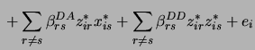
![\begin{displaymath}
L( \mathbf{E}, \mu, \sigma^2 \vert \mathbf{Y}, \mathbf{X}) =...
...ij} \phi(y_i \vert \mu + \mathbf{D}_j \mathbf{E}, \sigma^2 ) ]
\end{displaymath}](img254.png)